Background
I was first introduced to causal inference by Hernan and Robins (2021), in the summer of 2021 prior to starting my PhD. This book was tremendous and changed my thinking about “correlation doesn’t equal causation”.
From introductory science, as scientists, we are taught that correlation doesn’t equal causation. I had never questioned this until I was in my MSc program and started thinking about the association between lung cancer and smokers. Stellman et al. (2001) reported an odds ratio of 40.4 (95% CI: 21.8-79.6), which to me seemed high.
Now there are two ways to interpret this. On one hand, if we were a tobacco company we could argue that the 95% CI is pretty wide, indicating that the estimate is not that precise and the statistical method used must be wrong, etc (by etc, I mean whatever excuses you want to use). On the other hand, even at the lower limit an odds ratio of 21.8 is pretty damn high. In my opinion, this would require at the very least more investigation to determine “does smoking cause lung cancer?”
Common Ground
Prior to diving straight into the world of causal inference, we first need to set some common ground rules.
Keep in mind causal inference is a broad field and will be the subject of many subsequent posts, this is just an introductory post or wetting your beak if you will.
Confound It!
In order to get to the bottom of “does X cause Y?” we need to outlined some key methodological concepts. First, we need to outline what confounding is and clearly define what we mean.
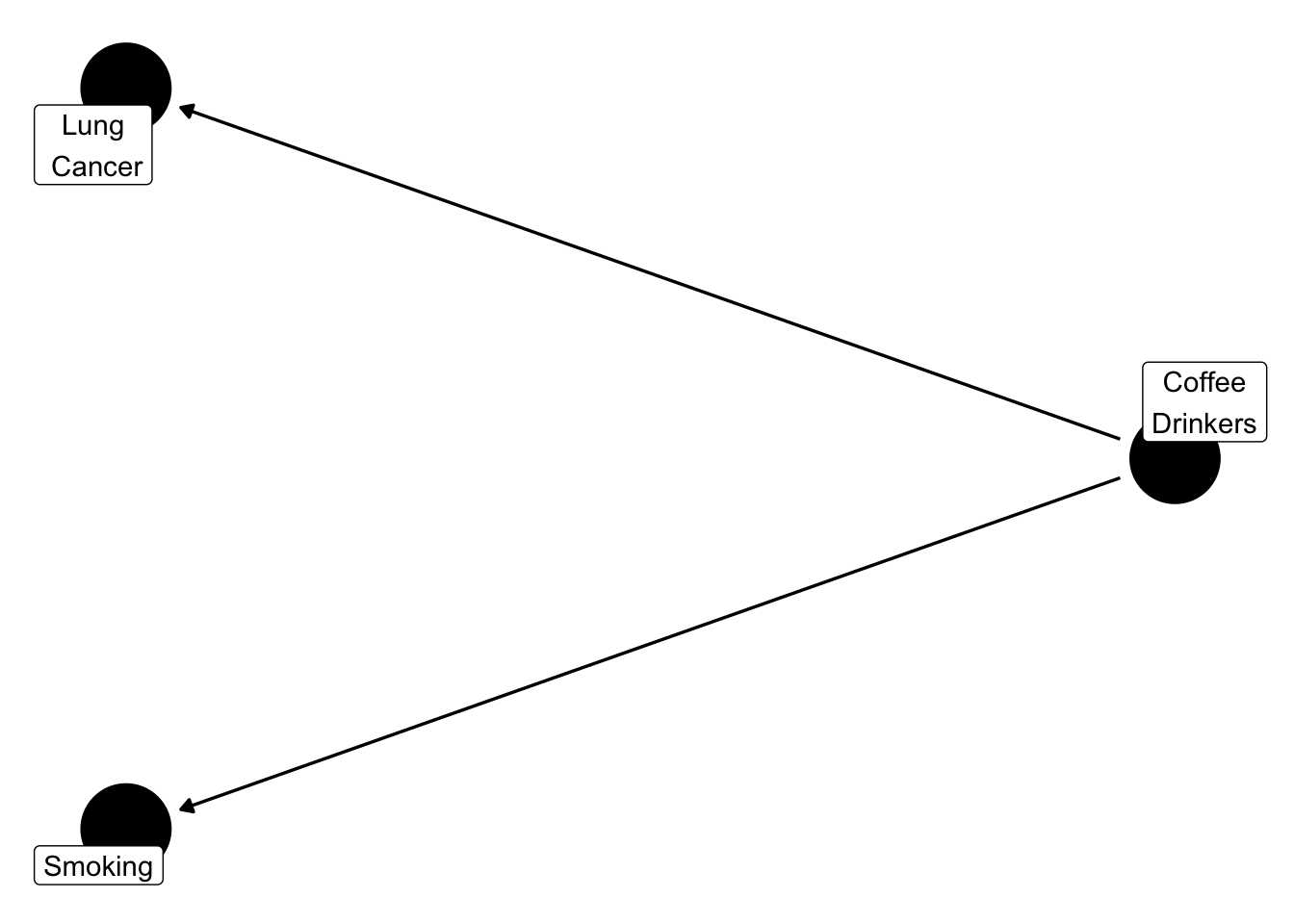
Different disciplines used different terminology, however confounding in clinical epidemiology refers to a variable that impacts both the exposure (i.e., smoking) and outcome (i.e., lung cancer). A useful way to visualize this is using directed acyclic graphs (DAGs). I’ll defer to Hernan and Robins (2021) for more detail about DAGs. However, the below illustrates what confounding is.

Figure 1 shows that coffee drinkers are associated with smoking. Logically, this makes sense because many smokers enjoy a cup of coffee with their cigarette. In fact, a lot of people enjoy coffee. A group of these people who are coffee lovers may also develop lung cancer. Based on this, you could say that people who drink coffee develop lung cancer. The question is, is this true? Or is it just that a lot of people like drinking coffee? Confounding bias, makes it difficult to tease out what coffee actually causes.
Randomized Controlled Trials (RCTs)
Randomized controlled trials are typically considered the gold standard in research. However, sometimes people forget why they are considered the gold standard. There are of course numerous reasons but I will touch on a few here. Firstly, an RCT is randomized meaning that patient’s are randomly assigned to one of the treatment arms. In theory, this is to ensure that characteristics are balanced between the treatment arms. By balancing characteristics, in theory, both observed and unobserved confounders are equal between the groups, making them exchangeable (aka similar).
Random is important to note here. There are different methods which are truly random, such as a random number generator, while there are others that are not.
For example, if you were picking players for a baseball team and wanted to assign people to two teams, team A & team B, how would you do it? Based on the color shirt they are wearing, hair color, eye color? None of those methods would be random.
Another key strength of RCTs is the nature of the intervention. For example, a well designed RCT will be very clear about what treatment is received by the participants and that all participants will receive the same treatment. Furthermore, one participant receiving a treatment won’t affect the other participant receiving treatment. It is also worth noting here that all participants in a RCT will receive some form of exposure (typically either treatment or placebo).
Observational Data
Observational data in research often gets a bad wrap. Since the gold standard is a RCT, people often view observational data as second-tier compared to an RCT. However, it all depends on how well the study is conducted. If the study is conducted rigorously, which is subjective but we will elaborate more below, then a study using observational data can be almost as good as an RCT.
Conditions Required for Causal Inference
Real-life is very complicated. For any method or analysis, such as designing a house, assumptions are required. This is is no different for causal inference. Key assumptions for causal inference include (Hernán 2012):
Exchangeability
Positivity
Consistency
No versions of treatment
No interference
Collectively, consistency, no versions of treatment and no interference have been referred to as the stable-unit-treatment-value assumption (SUTVA) (Hernán 2012).
Let’s break down these assumptions down one by one.
Exchangeability
Remember confounding from earlier? Well that pesky bias is back again to haunt us.
Recommend to pause here and re-read Section 2.1 if needed
The goal, although not always, of a lot of research is to compare two different exposures. An exposure could be a treatment, for example drug A to placebo, or to compare purple Popsicle eaters with water drinkers. An example always helps.
Let’s pretend we want to compare purple Popsicle eaters with water drinkers, to see if there is a difference in who is hungrier. Using an existing database of hungry people, we decide we want to compare these two groups of people. In the database, there are 591 people who have reported hunger.
| Demographic Variable | Purple Popsicle Eaters (n = 250) |
Water Drinkers (n = 341) |
|---|---|---|
| Age, mean (SD) | 9.18 (3.39) | 42.58 (22.03) |
| Female, n (%) | 190 (76.0%) | 145 (42.5%) |
Table 1 shows the average age and proportion of females in each of the two groups. Now, after looking at these two groups, you may think to yourself “Wait a minute…water drinks on average are 42 while purple Popsicle eaters are an average age of 9? These can’t possibly be compared!”.
Your inclination was right. These two groups are quite different and may vary in more ways than what is shown. This lack of similarity could be reworded as a lack of exchangeability. Luckily, there are fancy stats methods to fix this, which will be the topic of other posts.
While we can adjust for observed confounding, it is not possible to adjust for unobserved confounding. We simply don’t know about it, for example how many people in each group enjoy the taste of grape crush.
Positivity
Positivity refers to the condition that every individual has a greater than 0 probability of being assigned to each of the treatment levels (Hernan and Robins (2021), pp. 30). Logically, this makes sense because if we think about our purple Popsicle eaters and water drinks, if someone in that group had a less than 0 probability they couldn’t possibly be in that group!
Consistency
Consistency means that the observed outcome for every treated individual equals her outcome if she received treatment and that the observed outcome for every untreated individual equals her outcome if she had remained untreated, that is \(Y^a = Y\) for every individual with \(A = a\) (Hernan and Robins (2021), pp. 31).
On the surface, this seems intuitive but lets dive a little deeper. There are two components to consistency:
A precise definition of the counterfactual outcome \(Y^a\) via a detailed specification of the superscript \(a\) ( Hernan and Robins (2021)
Linkage of the counterfactual outcomes to the observed outcomes ( Hernan and Robins (2021))
The first bullet point is we essentially want to have a well defined intervention. If we think back to our purple Popsicles, we want to make sure that it is the same size, shape and brand that each participant receives. Doing this allows us to make sure that each participant is getting the same treatment.
For the second bullet point, remember we are using observational data for our purple Popsicle eaters. We have to make sure that for the analysis, we only treat people receiving our intervention (purple Popsicle eaters) as treated, or as Popsicle eaters, and the others as not Popsicle eaters.
No Versions of Treatment
As discussed in Section 3.3, we cannot have multiple versions of the same treatment. This would muddy our findings if we were giving different people different Popsicle. Plus, this would make it hard to determine the effect of purple Popsicles on hunger. Imagine, you gave some people a much bigger Popsicle than others. Of course they’d be less hungry!
No Interference
Interference here refers to the interference of the exposure. Exposure could be treatment, infectious disease or Popsicles. For our example, and most examples in this blog, the condition of no interference will be assumed to be met. Examples where this is not met is infectious disease studies (Hernan and Robins (2021)).
When to use Cause
Finally, all we wanted to do was get to use the word cause! Why? Because it’s important to use. If the above conditions hold, three main ones: exchangeability, positivity and consistency, then you can use the term cause. Besides, wouldn’t you want to know if Popsicles caused hunger?